A standard that fits everyone is a standard that fits half of them: for snow clearing as for pay.
Snow clearing in Karlskoga
In the small Swedish town of Karlskoga, the municipality cleared the main roads first after snowfall, then the footpaths and cycle paths. That sounded sensible, so for decades nobody questioned it. Then someone looked at the accident statistics separately for women and men: most winter injuries happened to people on foot, and most of those were women. When the town started clearing the footpaths first, accidents halved, and because the cost of treating the injuries had exceeded the cost of the winter road service, the town even saved money [1].
Nobody had decided to treat women worse. Someone had merely decided what the normal case was, and that was the person in a car. The same kind of decision sits inside every pay analysis, several times over, and it is as invisible as the ploughing schedule: someone has laid down what is being measured against, and everything that deviates from it has to explain itself.
Three places where someone decides what counts as normal
A pay analysis ends in a number. It looks as though it had been found in the dataset, when in fact it was calculated relative to something someone chose beforehand. That choice is made in three places: in the denominator of the percentage, in the category left out of the regression, and in the wage structure the decomposition assumes. None of the three appears in the report, although each of them shifts the result, some by several percentage points.
First place: the reference value for the gender pay gap
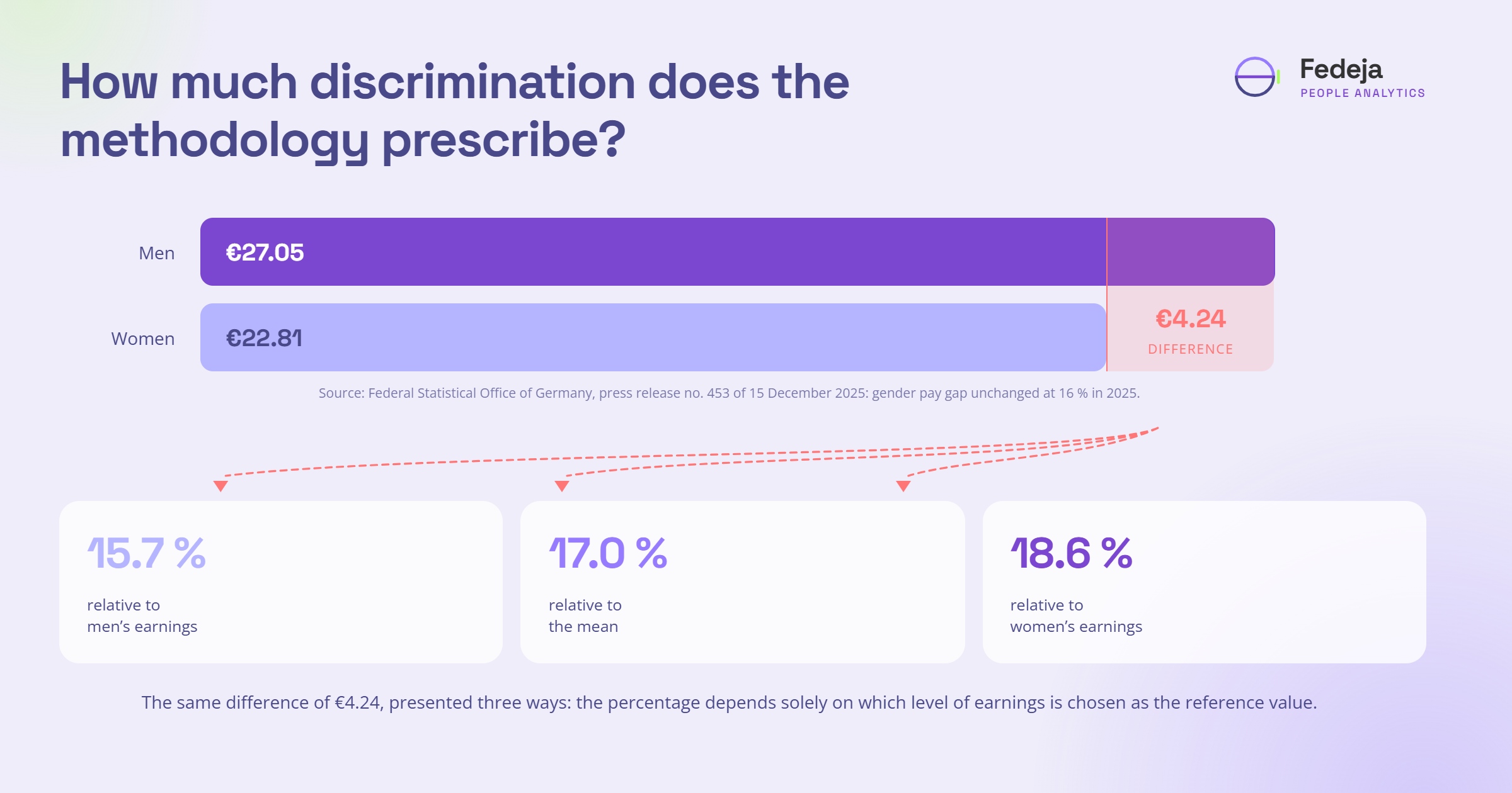
Two consultants, the same dataset, the same software: one reports 15.7%, the other 18.6%. Both calculated correctly, but they divided by different values. In 2025, women in Germany earned an average of 22.81 euros gross per hour, men 27.05 euros, a difference of 4.24 euros [2]. Divided by men’s earnings, that is 15.7%; divided by women’s earnings, 18.6%; measured against the mean of both groups, 17.0%.
All three answer a sensible question, just not the same one. The 15.7% says how much less women receive; the 18.6% says how far they are short of men’s level, and that is the figure for the cost of closing the gap. Which one is right depends on what the calculation is for. Statistics does not settle that.
The EU has taken the choice out of our hands: Article 3 of the Pay Transparency Directive puts the male average in the denominator [3]. Where this matters is Article 10: if the difference in a category is at least 5% and remains unexplained and unremedied, a joint pay assessment with the workers’ representatives follows. If men earn 5,250 euros and women 5,000, those 250 euros are 4.76% on the male base and exactly 5% on the female base: the same table, once unremarkable, once right on the threshold.
Under the Directive, the first calculation applies. The question is whether the internal tool does it the same way, and whether it is documented how the figure was calculated. Mean and median show the same pattern: Article 9 requires both, plus the pay quartiles. If they lie far apart, that tells you whether the gap sits across the board or at the top.
Second place: the person who does not appear
From here on, the reference decision is no longer just a denominator but the origin of the coordinate system. A regression can do nothing with words, so every categorical variable (location, function, pay grade, type of employment) is translated into zeros and ones. With 5 categories, 4 go into the model; one stays out and disappears into the intercept. From then on, every coefficient measures the distance to the category that was left out.
Which category that is, a human almost never decides. The software usually takes the first one in alphabetical or numerical order: your reference department is the reference because its name begins with A. Change the sort order and the table looks different, although model fit, R² and the adjusted overall gap stay where they were. What changes is the story someone reads off the table, and in a presentation the story is the result.
Put all the reference categories side by side (full-time, permanent contract, no career break, head office, reference pay grade) and together they describe a person. Their deviation is zero by construction; everyone else is the deviation.
In medicine, this construct at least has a name: since the 1970s, “Reference Man”, 70 kg, mid-twenties. Caroline Criado Perez has collected the consequences, from office temperature to the crash test dummy, a 1.75 m man weighing 78 kg: women face a higher risk of injury in frontal collisions because the car was tested on someone else [4].
Your pay system has a reference person too; it just has no name. A simple test: describe the person who scores full marks on every criterion in your job evaluation catalogue.
Third place: one line for everyone
The adjusted gap is almost always produced the same way: a multivariate regression across the whole workforce, pay explained by experience, function, location and pay grade, with sex as one variable among many. That is how I have seen it done in many projects. At the end stands a single coefficient, and that is reported as the pay gap. What this model assumes appears in no report: there is only one regression line, the same slope for women and men, just shifted downwards by a constant amount.
The model does not measure this point. It presupposes an answer to precisely the question that was supposed to be examined. A common line claims that a year of experience or a career step pays off for women exactly as it does for men. If that is not the case, the difference does not disappear; it is merely booked somewhere else: the model presses both groups onto one curve and pushes everything that does not fit into the sex coefficient.
Whose curve that is, group size decides. If men are in the majority, the common line essentially follows their trajectory, and women are described as the distance from it. Whatever sits in the slopes, say a flatter experience curve or a promotion that pays less, is invisible by construction. The gap appears more even than it is, and at the upper end, where the curves diverge most, the model underestimates the gap most.
Dark data: what appears in no table
Up to this point, the subject was decisions that shift the result. Now it is about what no model can show. The adjusted gap in 2025 stood at 6%; of the 4.24 euros, official statistics explain around 60% through measurable factors: part-time work 19%, occupation and sector 18%, requirement level of the job 13%. That leaves 1.71 euros remain [5].
Every control variable is formally gender-neutral and can itself be the result of disadvantage. Whoever controls for part-time work controls for unequally distributed care obligations; whoever controls for management level, for the promotions of the past 10 years; whoever controls for sector removes the historical devaluation of female-dominated occupations from the calculation. This is called overcontrol. The Federal Statistical Office itself writes that the adjusted gap must not be equated with pay discrimination, because data on career interruptions are missing. The 6% therefore mark an upper limit rather than a lower one.
David Hand calls this dark data [6]: the dangerous thing is not the missing value but the one whose absence nobody notices. The systems hold the outcome of the negotiation, never the conversation. Whoever applied internally and did not get the job does not appear. Whoever left because of the gap is no longer contained in it. And why a job sits in pay grade 9 rather than 11 is a question the regression does not ask; that is its input.
These things are unmeasured, not unexplained. What is unexplained appears as a residual and gets discussed; what is unmeasured does not appear in the report at all. That is the Karlskoga ploughing schedule: a norm that presents itself as a matter of course.
In closing
The question in the title can be calculated, and the answer regularly comes to several percentage points before causes or responsibility have even been discussed. Quantitative pay analyses remain the right tool all the same; they just are not neutral: every method is a chain of decisions, and each of those decisions has an addressee, the person who is made the zero point.
The consequence is unspectacular and is still rarely drawn: disclose the reference decisions, supply the alternative calculations, and name what is not in the data. In Karlskoga, after all, nobody changed the statistics either; someone simply asked who the ploughing schedule had been made for.
Frequently asked questions about pay analysis
1. Which figure counts for the Directive, the adjusted or the unadjusted one?
Under Article 9, the unadjusted difference is reported, as mean and median, together with the distribution across pay quartiles [3]. The adjusted figure is not prescribed anywhere. It helps internally with understanding, but it replaces neither the report nor the review by category.
2. What belongs in an alternative calculation?
At least three things: the gap with a different denominator, the regression model with separate lines for women and men, and the adjusted gap once with and once without the variables that can themselves be the result of disadvantage (part-time work, management level). If the results lie close together, the figure is robust. If they lie apart, that is the actual finding.
3. What to do when a category contains only a few women or only a few men?
Then a single person carries the average, and the figure swings from year to year without anything having changed. A regression delivers wide confidence intervals there, not a statement. It makes more sense to merge such groups or to justify them individually, and to say in the report from what group size the figure should be read at all.
Sources
• [1] FSG: Can Snow Clearing Be Sexist? (figures on the Karlskoga case). https://www.fsg.org/blog/can-snow-clearing-be-sexist/
• [2] Federal Statistical Office (Destatis), press release no. 453 of 15 December 2025: Gender Pay Gap 2025 unverändert bei 16 % (gender pay gap unchanged at 16%). https://www.destatis.de/DE/Presse/Pressemitteilungen/2025/12/PD25_453_621.html
• [3] Directive (EU) 2023/970 of 10 May 2023 (Pay Transparency Directive), in particular Articles 3, 9, 10 and 18. https://eur-lex.europa.eu/legal-content/EN/TXT/PDF/?uri=CELEX:32023L0970
• [4] Criado Perez, Caroline (2019): Invisible Women. Exposing Data Bias in a World Designed for Men, Chatto & Windus. (Reference Man, office temperature standard, crash test dummy, snow clearing in Karlskoga)
• [5] Federal Statistical Office (Destatis), Gender Pay Gap: Frequently asked questions (calculation formula, adjusted and unadjusted, limits of interpretation). https://www.destatis.de/DE/Themen/Arbeit/Verdienste/Verdienste-GenderPayGap/FAQ/_faq-gender-pay-gap.html
• [6] Hand, David J. (2020): Dark Data: Why What You Don’t Know Matters, Princeton University Press.
• [7] CMS Legal, EU Pay Transparency Directive: comprehensive reporting obligations for companies (deadlines and thresholds). https://cms.law/de/deu/legal-updates/eu-entgelttransparenzrichtlinie-umfassende-berichtspflichten-fuer-unternehmen